infotheory

Entropy ⇧

Entropy is a measure of uncertainty of a random variable. Greater the entropy, the more difficult it is to guess the value the random variable might take. It is function of the probability distribution rather than the actual values taken by the random variable, and it is estimated as follows -

where $H(X)$ denotes entropy of the random variable, $X$, the summation is over all values the random variable can take, $\forall x \in X$ and $p(x)$ or $p(X=x)$ denotes the probability that the random variable $X$ takes a particular value $x$. The logarithm is base 2 and so the measured entropy is in the unit of bits. Note that $0log0$ is taken to be $0$, and therefore adding new terms to $X$ with probability $0$ does not change its entropy.

Intuitively, for a given random variable, a uniform probability distribution over its values would result in the highest entropy since every value is equally likely, making it most difficult to guess. On the other hand, other ``peaky'' distributions such as Gaussian would have lower entropy since most of the probability mass is near the mean. From a communication systems perspective, where information theory had its origins, entropy can also be interpreted as the average number of bits required to efficiently encode the random variable. For example, a fair coin requires 1 bit (0-heads, 1-tails); a uniform distribution over 8 values of a random variable requires 3 bits, but a non-uniform distribution could possibly be encoded by smaller average number of bits by assigning shorter codes for more likely outcomes.

Benchmark ⇧

Entropy being a measure of uncertainty has an inverted-U relationship with the probability of success in Bernoulli trials. By generating 10000 data points for a range of values in $[0,1]$ for probability of heads in a simulated coin-toss experiment, we tested the entropy measure. Figure 1 below shows that we were able to produce the expected inverted-U relationship thereby meeting the benchmark for entropy.

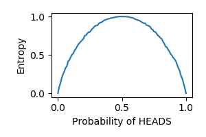
Fig. 1. Entropy benchmark. For different values of probability of heads in a coin flip, entropy should be an inverted-U curve

Mutual Information ⇧

One of the most widely used information theoretic measures is mutual information. It is a measure of the amount of information two random variables have about one another - it is a symmetric measure. The information one variable has about the other can be expressed as the reduction in uncertainty about one variable upon knowing the other i.e. the difference between entropy of the variable and the entropy given the other variable.

where $I(X;Y)$ is the mutual information between random variables $X$ and $Y$, $H(X)$ and $H(Y)$ are their respective entropies, and $H(X|Y)$ and $H(Y|X)$ are their corresponding conditional entropies. The conditional entropy can be estimated from the conditional probability density, which is related to their joint probability density. Upon writing out the entropy expressions about in terms of the marginal and joint densities we arrive at the following expression for mutual information between $X$ and $Y$

The relationship between the individual entropies, the conditional entropies and mutual information can be better understood using a Venn diagram, as shown in the figure below.

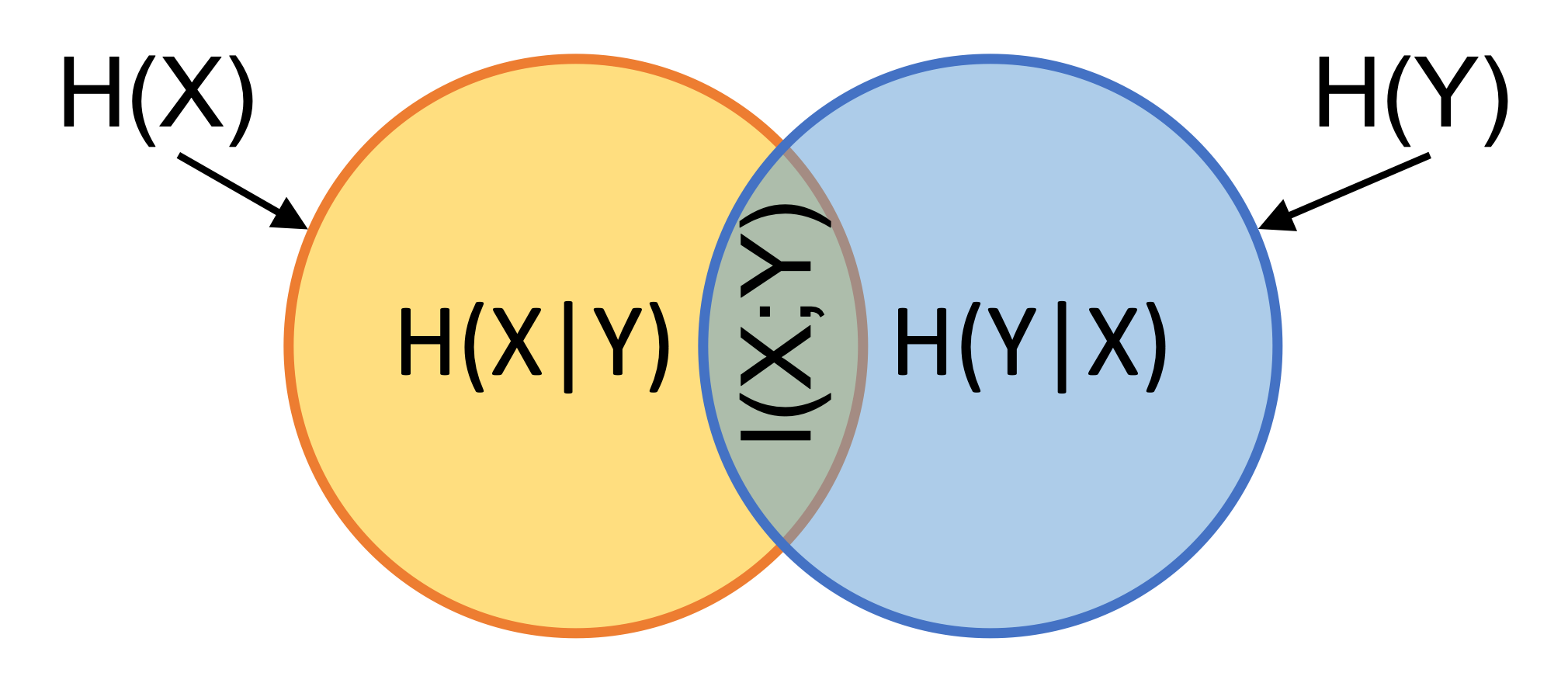
Fig 2. Relationship between indiavidual entropies and conditional entropies.

Mutual information can also be defined in terms of specific information. Specific information refers to information that one variable has, say $X$ about a specific value of another, say $Y$. Mutual information is then the total information averaged over all values of $Y$

where specifc information is given by

Benchmark ⇧

Mutual information, can be interpreted as a generalized measure of correlation. Irrespective of how they are correlated, if knowing the value of one variable is strongly predictive of the other, then mutual information is high (or 1, since we have normalized mutual information to be in $[0,1]$ for these analyses). Our first two benchmarks for mutual information evaluate this. First, we have two identical random variables showing near perfect information (Fig.3A). Second, a data distribution as shown in Fig.3B, when binned according to the grid shown on the figure, has perfect predictability of bins in one variable when the other is known. As expected, we see high levels of mutual information in this case too. Third, to the extent that thee two identical variables of the first case are noisy in their prediction of each other, we see a reduction in the amount of information. Also, demonstrated successfully in Fig.3C. Finally, when two variables are in no way predictive of each other, evaluated by two independent uniform random variables, the mutual information as expected is near zero (Fig.3D).

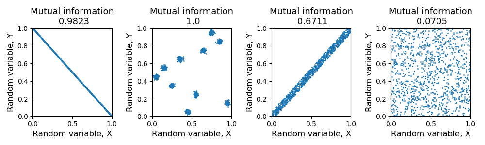
Fig 3. Mutual information benchmark. [A] Normalized mutual information is ~1 for identical variables [B] Normalized mutual information is ~1 for variables where bins even though there is no direct correlation between x and y, knowledge of x is highly indicative of y [C] Normalized mutual information is lower for noisy identical variables and low for random variables [D] Normalized mutual information is ~0 for uniform random variables

Demo ⇧

While the code for the benchmark above also acts as a demo on how this package can be used to estimate mutual information, this demo shows a further use of the mutual information measure method. Using this package, mutual information can also be estimated over time to see how information encoded in one variable about another changes over time. This is achived by repeating the analyses over each time point in the data, by providing the same mutual information method used above it.mutual_info() but providing the data from only that time point. Figure 4 below demonstrates such an analyses over a simulated system where information in the reecorded data about the stimulus is measured over time.

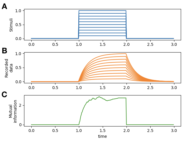
Fig 4. Mutual information over time. [A] Stimuli with varying amplitudes provided over time [B] Simulated recorded data that has been designed to encode the stimulus [C] Mutual information measured in time captures the designed encoding of stimulus by the data

Partial Information Decomposition ⇧

The extension of mutual information to the multivariate case is non-trivial because with multiple variables, it becomes crucial to understand the structure of the dependencies between them. In a multivariate setting, if the different variables are separated into source and target variables, the total mutual information between these sources and the `target' variable can be decomposed into its non-negative constituents, namely, unique information from each source, redundant information that the sources provide, and synergistic information due to combined information from multiple sources [1]. Consider two sources of information (two random variables) $X1$ and $X2$, about the random variable $Y$. If $X=\{X1,X2\}$, the total mutual information $I(X;Y)$ can be written as follows

where $U$ denotes unique information, $R$ denotes redundant information and $S$ denotes synergistic information from these sources about $Y$. The decomposition can be better understood when visualized as a Venn diagram as shown in figure 5. Naturally, with more than two sources, redundant and synergistic information will be available for the all combinations of the different sources. Furthermore, with three sources, more overlapping information atoms exist such as the overlap between source 3 and the synergistic combination of 1 and 2, and the like. This package currently implements partial information decomposition for the two source and three source scenarios. Note that each source could be a multi-dimensional random variable.

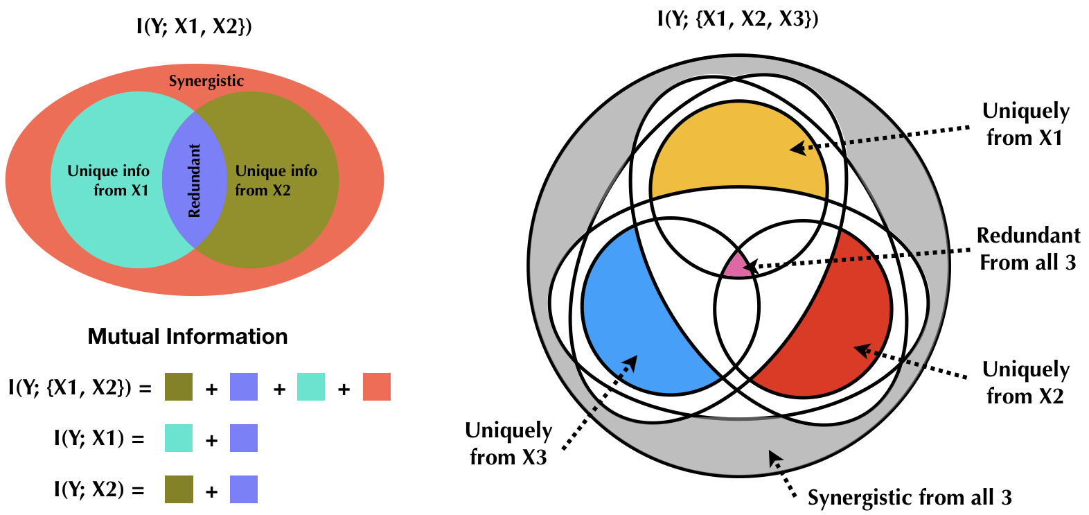
Fig 5. Relationship between total information and PID components in the 2 source and 3 source cases. The entire venn diagram represents the total information. The 3 source decomposition gives a more generic picture, because it shows additional overelapping slices that do not exist in the 2 source case such as the redundant overelap between the synergistic combination of two sources and the unique contribution of the third, and so on. See [1] for a thorough description of all slices in the Venn diagram.

Redundant Information ⇧

The sum of the minimum value of specific information each source provides is defined as the redundant information from the two sources. In other words, continuing the $(\{X1,X2\},Y)$ example, for each value of $Y$, the specific information $X1$ and $X2$ provide is independently computed, its minimum is found and this values is summed across all values of $Y$.

Unique Information ⇧

The amount of information that each source uniquely contributes, the unique information from that source, is estimated as the difference between the mutual information between that source and the `target' variable and the redundant information estimated as shown in the previous section. This is also apparent from the Venn diagram representation shown in figure 5.

Synergistic Information ⇧

The information about $Y$ that does not come from any of the sources individually, but due to the combined knowledge of multiple sources, is synergistic information. For example, in an XOR operation, knowledge about any one of the inputs is insufficient to predict the output accurately, however, knowing both inputs will determine the output. In contrast, in an AND gate, merely knowing that one of the inputs is $False$ can lead to the conclusion that the output is $False$. Again, based on the Venn diagram in figure 5, synergistic information from sources $X={X1,X2}$ about $Y$ can be determined based on total, unique and redundant information components as follows

Benchmark ⇧

Discrete data ⇧

For an XOR gate, by its definition each input provides no unique information, and hence no redundant information. The output of an XOR gate can only be inferred through the synergistic information of both inputs combined. This should show up in the partial information decomposition of the total mutual information between inputs and outputs in an XOR gate. However, in an AND gate the output can be determined to be 0, if one of the inputs is 0, and so the other input is redundant in that case; and an output of 1 can only be inferred if both information from both inputs are together known to be 1. This also can be brought out from partial information decomposition. See Table 1. in [2] for corroboration of numbers shown below.

2-input logical AND
total_mi = 0.8112781244591328
redundant_info = 0.3112781244591328
unique_1 = 5.551115123125783e-17
unique_2 = 5.551115123125783e-17
synergy = 0.49999999999999994

2-input logical XOR
total_mi = 1.0
redundant_info = 0.0
unique_1 = 0.0
unique_2 = 0.0
synergy = 1.0

3-input logical AND
total_mi = 0.5435644431995963
mi_12 = 0.29356444319959635
mi_13 = 0.29356444319959635
mi_23 = 0.29356444319959635
mi_1 = 0.1379253809700299
mi_2 = 0.1379253809700299
mi_3 = 0.1379253809700299
redundant_info = 0.1379253809700299
redundant_12 = 0.1379253809700299
redundant_13 = 0.1379253809700299
redundant_23 = 0.1379253809700299
unique_1 = 0.0
unique_2 = 0.0
unique_3 = 0.0
synergy = 0.24999999999999983
synergy_12 = 0.15563906222956644
synergy_13 = 0.15563906222956644
synergy_23 = 0.15563906222956644

3-input Even parity
total_mi = 1.0
redundant_info = 0.0
redundant_12 = 0.0
redundant_13 = 0.0
redundant_23 = 0.0
unique_1 = 0.0
unique_2 = 0.0
unique_3 = 0.0
synergy = 1.0
synergy_12 = 0.0
synergy_13 = 0.0
synergy_23 = 0.0

Continuous data ⇧

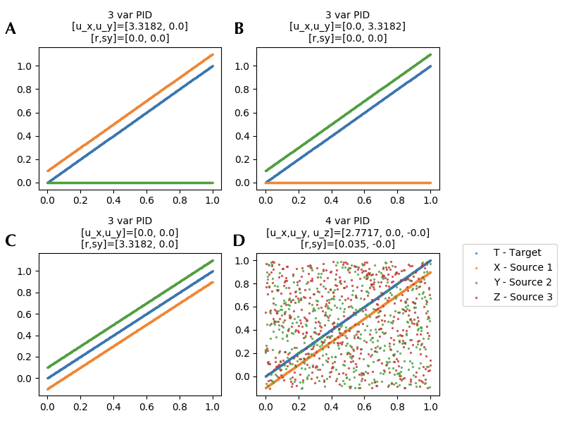
Fig. 6. PID with continuous variables S, X and Y, where X and Y are considered sources and S is the target. [A] When S and X vary identically PID shows that the total information is equal to the unique contributions of S. [B] Similarly when S and Y vary identically, the total information is equivalent to the unique information from Y. [C] Moreover, when both X and Y vary identically with S, the total information is equal to the redundant information from X and Y, and finally [D] an illustration of 4 variable decomposition (3 sources and 1 target) where one source primarily provides the information.

References⇧

1. Williams, P. L., & Beer, R. D. (2010). Non-negative decomposition of multivariate information. arXiv preprint arXiv:1004.2515.
2. Timme, N., Alford, W., Flecker, B., & Beggs, J. M. (2014). Synergy, redundancy, and multivariate information measures: an experimentalist’s perspective. Journal of computational neuroscience, 36(2), 119-140.
3. Schreiber, T. (2000). Measuring information transfer. Physical review letters, 85(2), 461.
4. Williams, P.L. and Beer, R.D., 2011. Generalized measures of information transfer. arXiv preprint arXiv:1102.1507.